A tutorial on running network twin analyses

twin modelling

genetics

network analysis

Published

July 12, 2025

In my 2024 paper “Comparing factor and network models of cognitive abilities using twin data”, Robert Plomin and I used a novel network twin analysis to estimate genetic partial correlations among cognitive abilities. Below is a tutorial for running a similar analysis using the GFF example dataset from the umx package.

Knyspel, J. & Plomin, R. (2024). Comparing factor and network models of cognitive abilities using twin data. Intelligence, 104, 101833. https://doi.org/10.1016/j.intell.2024.101833
Open Access Download PDF View Preregistration

Feel free to reach out to me with any queries you have!

Our analysis comprises three key steps:

Run a multivariate twin model on one half of the data to estimate genetic and environmental covariance matrices.
Use those genetic covariance matrices as the input for initial network analyses.
Run a unified network twin model on the other half of the data to cross-validate our network structures.

Setup

# Load required packages
library(psychonetrics)
library(qgraph)
library(OpenMx)
library(umx)

For this tutorial we will use the GFF dataset from the umx package. It includes five variables: general family functioning (gff), family conflict (fc), quality of life (qol), general happiness (hap), and life satisfaction (sat). For information, see ?GFF.

# Load example data
data(GFF)

# Generate indices for 50/50 sample split
set.seed(12345)
ind <- sample(seq_len(nrow(GFF)), size = floor(0.5*nrow(GFF)))

# Subset and split MZ and DZ data
dzData1 <- subset(GFF[ind,], zyg_2grp == "DZ")
mzData1 <- subset(GFF[ind,], zyg_2grp == "MZ")
dzData2 <- subset(GFF[-ind,], zyg_2grp == "DZ")
mzData2 <- subset(GFF[-ind,], zyg_2grp == "MZ")

# Specify variables for analysis
selDVs <- c("gff", "fc", "qol", "hap", "sat")

1) Multivariate twin model

Our first step is to run a generic multivariate twin model to estimate genetic and environmental covariance matrices. The umxACEv() function is a good option for this model. For the sake of simplicity, only an AE model is included here. In practice, it is important to compare ACE, AE, CE and E models to arrive at the best fitting one.

# Run ACE model
ACE <- umxACEv(selDVs = selDVs, dzData = dzData1, mzData = mzData1, sep = "_T")

# Reduce model to AE model
AE <- umxModify(lastFit = ACE, update = ACE$top$C$labels, name = "AE")

If the model is producing status codes 5 or 6, it is first worth re-running it with mxTryHard() or using a different optimizer via umx_set_optimizer(). If it is still producing these status codes, we can check if it is locally identified.

# Check if model is locally identified
mxCheckIdentification(AE)$status

If the model is not locally identified, it would benefit from being made simpler, perhaps by removing the variables with the smallest twin correlations one at a time. Once we have an acceptable model, we can extract the genetic and non-shared environmental covariance matrices and perform some additional checks to ensure they are suitable for the next step.

# Extract A and E matrices
A <- AE$top$A$values
E <- AE$top$E$values

# Check if matrices are symmetric
isSymmetric(A)
isSymmetric(E)

# Check if eigenvalues are non-negative
sum(eigen(A)$values >= 0) > 0
sum(eigen(E)$values >= 0) > 0

If a matrix is not symmetric or has any negative eigenvalues, this means it is not positive semi-definite, which will present a problem for network analysis. In this case, it is worth trying umxACE() instead of umxACEv(). This function will ensure that the matrices are positive semi-definite, although it is more easily subject to status codes 5 and 6. If we are happy with the matrices, we can then begin our network analysis.

2) Initial network analysis

Here we will use the covariance matrices from step 1 to estimate network models sparsified using p-value thresholding and stepwise BIC selection. An alternative approach to sparsification here would be regularisation. First, we fit a saturated network model.

# Run saturated network models
networkA <- ggm(covs = A, nobs = length(ind)) |>
  runmodel()
networkE <- ggm(covs = E, nobs = length(ind)) |>
  runmodel()

If runmodel() gives us a warning message here that (1) the information matrix is not positive semi-definite, (2) parameters were estimated near to their bounds or (3) the model failed to converge, it is first worth trying a different optimizer (see ?runmodel). If this does not work, it is worth proceeding to the next step anyway, which is sparsifying the models. This can be enough to solve the issue.

# Sparsify network models
sparseA <- networkA |>
  prune() |>
  stepup() |>
  runmodel()
sparseE <- networkE |>
  prune() |>
  stepup() |>
  runmodel()

If we are still receiving warning messages after sparsifying the models, they might benefit from being made simpler, perhaps by removing the least heritable variables one at a time. The warning message about the information matrix being not positive semi-definite might occasionally be a false flag, especially if no other warning messages are given, the model has plausible partial correlations (not equal to or approaching 1 or -1) and produces the same log-likelihood when run multiple times.

# Check log-likelihood of sparsified models
sparseA@fitmeasures$logl
sparseE@fitmeasures$logl

When the sparsified model produces no warning messages or we are happy that the warning messages can be ignored, we can extract and plot our networks of partial correlations.

# Extract network model estimates
omegaA <- getmatrix(sparseA, "omega")
deltaA <- getmatrix(sparseA, "delta")
omegaE <- getmatrix(sparseE, "omega")
deltaE <- getmatrix(sparseE, "delta")

# Plot networks
par(mfrow = c(1,2))
qgraph(omegaA, labels = selDVs, layout = "spring", title = "A")
qgraph(omegaE, labels = selDVs, layout = "spring", title = "E")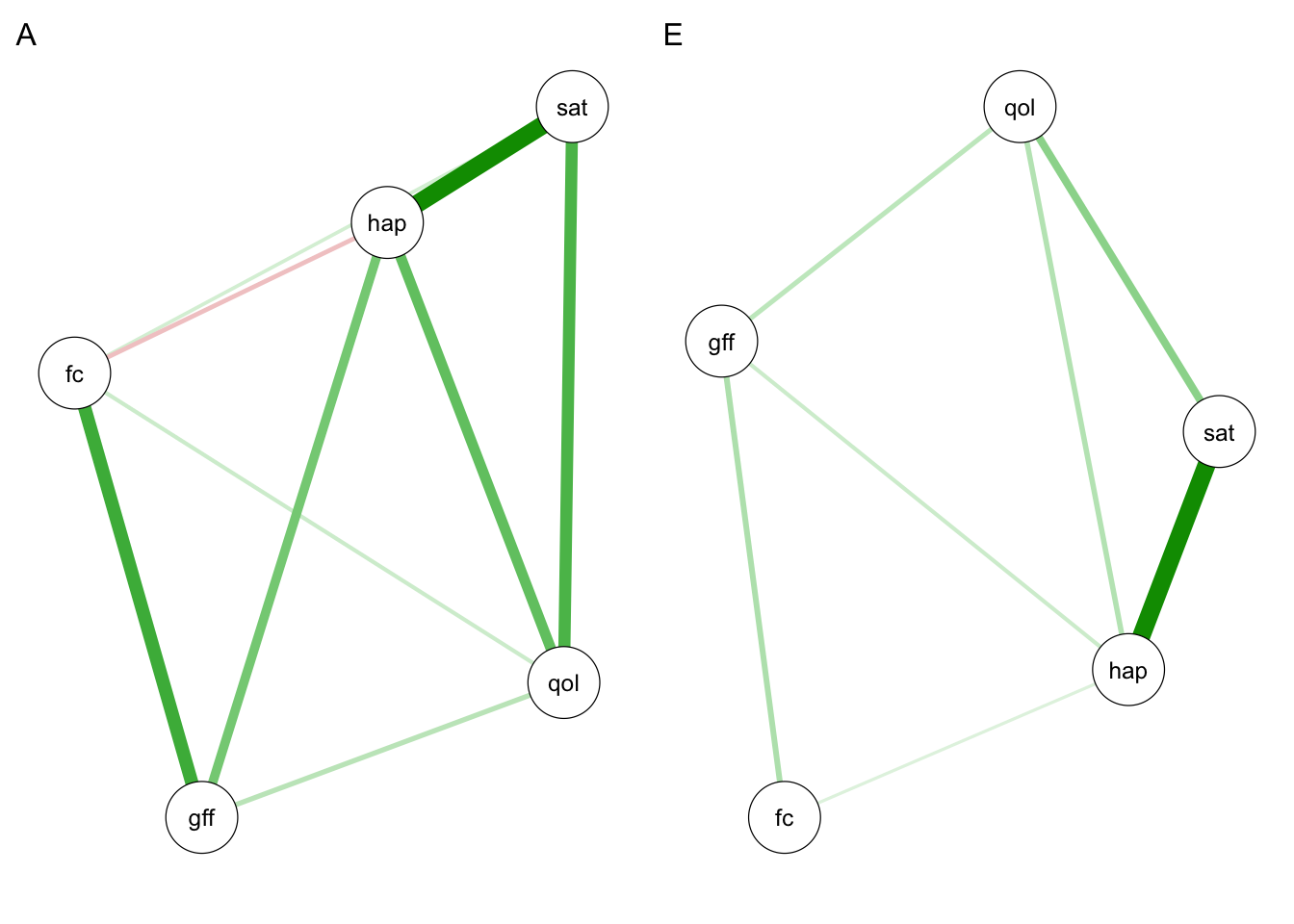

3) Network twin model

Our third and final step is to estimate a unified network twin model that simultaneously models A and E as partial correlation matrices. We does this in the other half of the sample as a form of cross-validation, using the partial correlation values from step 2. Estimating a unified model like this has the benefits of allowing for model fit statistics to be calculated and bootstrapping to be performed. The model can be flexibly adapted to include a C component or to model only one of the components (e.g. A) as a partial correlation matrix if desired.

# Specify additional variables for model
selVars <- xmu_twin_upgrade_selDvs2SelVars(selDVs, "_T", 2)
nVar <- length(selDVs)

# Create base components for network twin model
networkAE <- xmu_make_TwinSuperModel("base", mzData2, dzData2, selDVs, sep = "_T")

# Built additional model components
networkAE.top <- mxModel(networkAE$top,
                    
  # DZ twin similarity                  
  umxMatrix("dzAr", "Full", 1, 1, free = FALSE, values = 0.5),
  
  # Combined covariances
  mxAlgebra(name = "AE", A + E),
  mxAlgebra(name = "hA", dzAr %x% A),
  
  # Expected covariances by zygosity
  mxAlgebra(name = "expCovMZ", rbind(cbind(AE,A), cbind(A,AE)), dimnames = list(selVars, selVars)),
  mxAlgebra(name = "expCovDZ", rbind(cbind(AE,hA), cbind(hA,AE)), dimnames = list(selVars, selVars)),
  
  # Identity matrix
  umxMatrix("I", "Iden", nVar, nVar),
  
  # Additive genetic network
  # Using results from step 2 as starting values and constraints
  umxMatrix("deltaA", "Diag", nVar, nVar, free = TRUE, values = deltaA),
  umxMatrix("omegaA", "Symm", nVar, nVar, free = omegaA != 0, values = omegaA),
  mxAlgebra(name = "A", deltaA %*% (solve(I-omegaA)) %*% deltaA),
  
  # Non-shared environmental network
  # Using results from step 2 as starting values and constraints
  umxMatrix("deltaE", "Diag", nVar, nVar, free = TRUE, values = deltaE),
  umxMatrix("omegaE", "Symm", nVar, nVar, free = omegaE != 0, values = omegaE),
  mxAlgebra(name = "E", deltaE %*% (solve(I-omegaE)) %*% deltaE)
                    
)

If you’re familiar with twin modelling, you might recognise that this model is almost identical to a typical multivariate model, such as the one used in step 1. The only difference is that the A and E covariances are estimated as \(\Delta(I-\Omega)^1\Delta\), where \(\Omega\) is our matrix of partial correlations (i.e. our network) and \(\Delta\) is a diagonal scaling matrix.

# Run model
networkAE <- mxModel(networkAE, networkAE.top) |>
  mxTryHard()

Running base with 31 parameters


Beginning initial fit attempt

Running base with 31 parameters


 Lowest minimum so far:  62052.4209260318


Solution found


 Solution found!  Final fit=62052.421 (started at 62139.657)  (1 attempt(s): 1 valid, 0 errors)

 Start values from best fit:

38.5901046282982,-13.3668862571515,7.79648548997818,23.0176317324942,27.5693472922932,2.3899653420867,1.52239944488783,0.422499190051456,1.19669551190486,1.6426988234192,0.399341758597834,0.228012532206816,0.0894203608933922,0.265396356210378,-0.0765255904052195,0.226277141928524,0.0835354165144468,0.2904105960134,0.617672418713217,3.32098697034475,1.12335463995123,0.79080370482218,2.71605543224306,2.916173253324,0.149863900290934,0.142694075534241,0.0320753643951324,0.0339918408374545,0.163667794780947,0.194483670327578,0.636627915320457

As with step 1, if the model is producing status codes 5 or 6, it is worth trying a different optimizer via umx_set_optimizer(). If it is failing to converge but has valid attempts, we can try more attempts (see ?mxTryHard) or again try a different optimizer. If the model is still facing problems, we should check if it is locally identified.

# Check model is locally identified
mxCheckIdentification(networkAE)$status

If the model is not locally identified, it would benefit from being made simpler, either by removing variables or removing C components if they have been included. Once we are happy with the model, we can first get the summary output, using mxRefModels() to give us model fit statistics.

# Summarise model with fit statistics
summary(networkAE, refModels = mxRefModels(networkAE, TRUE))

Running Saturated base with 130 parameters

Running Independence base with 40 parameters

Summary of base 
 
free parameters:
             name      matrix   row    col     Estimate  Std.Error A
1  expMean_gff_T1 top.expMean means gff_T1  38.59010463 0.10758664  
2   expMean_fc_T1 top.expMean means  fc_T1 -13.36688626 0.04914363  
3  expMean_qol_T1 top.expMean means qol_T1   7.79648549 0.02341602  
4  expMean_hap_T1 top.expMean means hap_T1  23.01763173 0.09787622  
5  expMean_sat_T1 top.expMean means sat_T1  27.56934729 0.11466345  
6     deltaA_r1c1  top.deltaA     1      1   2.38996534 0.16941191  
7     deltaA_r2c2  top.deltaA     2      2   1.52239944 0.04542257  
8     deltaA_r3c3  top.deltaA     3      3   0.42249919 0.04299013  
9     deltaA_r4c4  top.deltaA     4      4   1.19669551 0.19787435  
10    deltaA_r5c5  top.deltaA     5      5   1.64269882 0.15546657  
11    omegaA_r2c1  top.omegaA     1      2   0.39934176 0.05343461  
12    omegaA_r3c1  top.omegaA     1      3   0.22801253 0.12764957  
13    omegaA_r3c2  top.omegaA     2      3   0.08942036 0.06840587  
14    omegaA_r4c1  top.omegaA     1      4   0.26539636 0.10802537  
15    omegaA_r4c2  top.omegaA     2      4  -0.07652559 0.08920932  
16    omegaA_r4c3  top.omegaA     3      4   0.22627714 0.16201806  
17    omegaA_r5c2  top.omegaA     2      5   0.08353542 0.05753107  
18    omegaA_r5c3  top.omegaA     3      5   0.29041060 0.14710234  
19    omegaA_r5c4  top.omegaA     4      5   0.61767242 0.08114828  
20    deltaE_r1c1  top.deltaE     1      1   3.32098697 0.08473517  
21    deltaE_r2c2  top.deltaE     2      2   1.12335464 0.03061927  
22    deltaE_r3c3  top.deltaE     3      3   0.79080370 0.02173415  
23    deltaE_r4c4  top.deltaE     4      4   2.71605543 0.08532173  
24    deltaE_r5c5  top.deltaE     5      5   2.91617325 0.08425109  
25    omegaE_r2c1  top.omegaE     1      2   0.14986390 0.03675147  
26    omegaE_r3c1  top.omegaE     1      3   0.14269408 0.03682949  
27    omegaE_r4c1  top.omegaE     1      4   0.03207536 0.03125440  
28    omegaE_r4c2  top.omegaE     2      4   0.03399184 0.03102033  
29    omegaE_r4c3  top.omegaE     3      4   0.16366779 0.04011893  
30    omegaE_r5c3  top.omegaE     3      5   0.19448367 0.04072182  
31    omegaE_r5c4  top.omegaE     4      5   0.63662792 0.02206175  

Model Statistics: 
               |  Parameters  |  Degrees of Freedom  |  Fit (-2lnL units)
       Model:             31                  13160              62052.42
   Saturated:            130                  13061              61857.59
Independence:             40                  13151              66688.44
Number of observations/statistics: 1593/13191

chi-square:  χ² ( df=99 ) = 194.8301,  p = 3.12413e-08
Information Criteria: 
      |  df Penalty  |  Parameters Penalty  |  Sample-Size Adjusted
AIC:       35732.42               62114.42                 62115.69
BIC:      -34981.18               62281.00                 62182.51
CFI: 0.9797863 
TLI: 0.9816239   (also known as NNFI) 
RMSEA:  0.02465048  [95% CI (0.01845002, 0.03066522)]
Prob(RMSEA <= 0.05): 1
timestamp: 2025-07-18 09:58:15 
Wall clock time: 0.555613 secs 
optimizer:  SLSQP 
OpenMx version number: 2.22.7 
Need help?  See help(mxSummary)

We can then extract and plot our networks of partial correlations, similar to step 2.

# Extract network model estimates
omegaA2 <- networkAE$top$omegaA$values
deltaA2 <- networkAE$top$deltaA$values
omegaE2 <- networkAE$top$omegaE$values
deltaE2 <- networkAE$top$deltaE$values

# Plot networks
par(mfrow = c(1,2))
qgraph(omegaA2, labels = selDVs, layout = "spring", title = "A")
qgraph(omegaE2, labels = selDVs, layout = "spring", title = "E")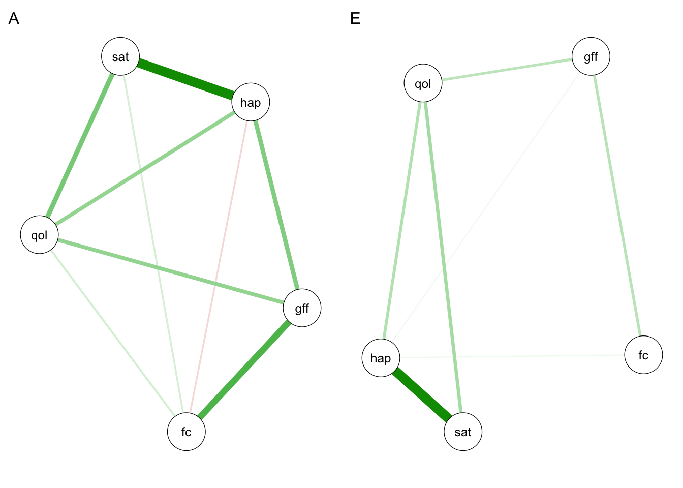

Comparing steps 2 and 3

Since we used cross-validation here, it is useful for us to compare the consistency in results between our initial network analysis (step 2) and subsequent network twin model (step 3). The more consistent the results are across the two halves of the data, the more confident we can be that our estimated networks are robust. There are many metrics we could use to assess consistency. Here I include root mean squared deviation (RMSD) and \(r^2\) as two examples.

# Create function to calculate RMSD and r2 between symmetric matrices
rmsd <- function(A,B) {
  lowerA <- A[lower.tri(A)][A[lower.tri(A)] > 0]
  lowerB <- B[lower.tri(B)][B[lower.tri(B)] > 0]
  list(A = lowerA,
       B = lowerB,
       RMSD = sqrt(mean((lowerA-lowerB)^2)),
       r2 = cor(lowerA,lowerB)^2)
}

# Calculate RMSD and r2 between network estimates from two methods
rmsd(omegaA2, omegaA)

$A
[1] 0.39934176 0.22801253 0.26539636 0.08942036 0.08353542 0.22627714 0.29041060
[8] 0.61767242

$B
[1] 0.40582666 0.13180353 0.27225009 0.09637653 0.08150718 0.31540359 0.36767353
[8] 0.56619175

$RMSD
[1] 0.05696605

$r2
[1] 0.878616

rmsd(omegaE2, omegaE)

$A
[1] 0.14986390 0.14269408 0.03207536 0.03399184 0.16366779 0.19448367 0.63662792

$B
[1] 0.15286517 0.12333334 0.09418465 0.06419384 0.14008567 0.21996795 0.56211580

$RMSD
[1] 0.04125044

$r2
[1] 0.9799998

As we can see, the results of our non-shared environment networks are more consistent than our genetic networks, although overall both perform well. Nice!

Thanks for reading! Feel free to reach out to me if you have any questions

Session Info

sessionInfo()

R version 4.5.0 (2025-04-11)
Platform: aarch64-apple-darwin20
Running under: macOS Sequoia 15.5

Matrix products: default
BLAS:   /Library/Frameworks/R.framework/Versions/4.5-arm64/Resources/lib/libRblas.0.dylib 
LAPACK: /Library/Frameworks/R.framework/Versions/4.5-arm64/Resources/lib/libRlapack.dylib;  LAPACK version 3.12.1

locale:
[1] en_US.UTF-8/en_US.UTF-8/en_US.UTF-8/C/en_US.UTF-8/en_US.UTF-8

time zone: Europe/London
tzcode source: internal

attached base packages:
[1] stats     graphics  grDevices utils     datasets  methods   base     

other attached packages:
[1] umx_4.21.0           OpenMx_2.22.7        qgraph_1.9.8        
[4] psychonetrics_0.13.1

loaded via a namespace (and not attached):
  [1] Rdpack_2.6.4        mnormt_2.1.1        pbapply_1.7-2      
  [4] gridExtra_2.3       fdrtool_1.2.18      rlang_1.1.6        
  [7] magrittr_2.0.3      compiler_4.5.0      mgcv_1.9-1         
 [10] png_0.1-8           systemfonts_1.2.3   vctrs_0.6.5        
 [13] reshape2_1.4.4      IsingSampler_0.2.4  combinat_0.0-8     
 [16] quadprog_1.5-8      stringr_1.5.1       pkgconfig_2.0.3    
 [19] crayon_1.5.3        fastmap_1.2.0       backports_1.5.0    
 [22] pbivnorm_0.6.0      rmarkdown_2.29      pracma_2.4.4       
 [25] nloptr_2.2.1        purrr_1.0.4         xfun_0.52          
 [28] jsonlite_2.0.0      jpeg_0.1-11         psych_2.5.3        
 [31] parallel_4.5.0      lavaan_0.6-19       cluster_2.1.8.1    
 [34] R6_2.6.1            stringi_1.8.7       RColorBrewer_1.1-3 
 [37] boot_1.3-31         rpart_4.1.24        numDeriv_2016.8-1.1
 [40] Rcpp_1.0.14         iterators_1.0.14    knitr_1.50         
 [43] base64enc_0.1-3     polycor_0.8-1       Matrix_1.7-3       
 [46] splines_4.5.0       nnet_7.3-20         igraph_2.1.4       
 [49] tidyselect_1.2.1    rstudioapi_0.17.1   abind_1.4-8        
 [52] yaml_2.3.10         MuMIn_1.48.11       codetools_0.2-20   
 [55] admisc_0.38         lattice_0.22-6      tibble_3.2.1       
 [58] plyr_1.8.9          evaluate_1.0.3      foreign_0.8-90     
 [61] RcppParallel_5.1.10 xml2_1.3.8          pillar_1.10.2      
 [64] DiagrammeR_1.0.11   checkmate_2.3.2     foreach_1.5.2      
 [67] stats4_4.5.0        reformulas_0.4.1    generics_0.1.4     
 [70] VCA_1.5.1           ggplot2_3.5.2       scales_1.4.0       
 [73] minqa_1.2.8         xtable_1.8-4        gtools_3.9.5       
 [76] glue_1.8.0          Hmisc_5.2-3         tools_4.5.0        
 [79] data.table_1.17.4   lme4_1.1-37         visNetwork_2.1.2   
 [82] cowplot_1.1.3       grid_4.5.0          tidyr_1.3.1        
 [85] rbibutils_2.3       colorspace_2.1-1    nlme_3.1-168       
 [88] GA_3.2.4            htmlTable_2.4.3     Formula_1.2-5      
 [91] cli_3.6.5           kableExtra_1.4.0    textshaping_1.0.1  
 [94] optimx_2025-4.9     viridisLite_0.4.2   svglite_2.2.1      
 [97] dplyr_1.1.4         corpcor_1.6.10      glasso_1.11        
[100] gtable_0.3.6        digest_0.6.37       htmlwidgets_1.6.4  
[103] farver_2.1.2        htmltools_0.5.8.1   lifecycle_1.0.4    
[106] MASS_7.3-65